As we talked about previously, usually the 'sig.level' = 0.05 and 'power' = 0.8. In an ideal world, the power will be 0.8, which means that you have an 80% chance of detecting a significant result if one exists.

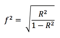
Calculate effect size:

The effect size for multiple regression is calculated from the model's R² value using the following equation:

This is fairly straight forward to calculate if you have pilot data, as you can caluclate it from the model output by dividing the group Sum of Squares by the residudal Sum of Squares. In R, first we can fit continuous variables x and y to a linear regression model and ask R for a summary of the model:

Once we have the summary, we can see the Multiple R² value at the bottom. So, if we tell R what the R² value is from this (0.04839) we can calculate the F² value straightforwardly:

Cohen (1988) suggests f² values of 0.02, 0.15, and 0.35 represent small, medium, and large effect sizes, respectively.

If you have a multiple regression model, the formula is slightly different, and a little more complicated to explain and to calculate:

In this equation, 'B' refers to the variable of interest (i.e., the variable you wish to find the effect size for) and 'A' is the sum of the variation accounted for by all the other variables in the model (relative to a null model). So, R²_AB is the sum of all of the variance accounted for by all of the variables (relative to a null model), and R²_B is the unique variance accounted for by your variable of interest (relative to a null model). Confused? Well, let's have a go at this in R.

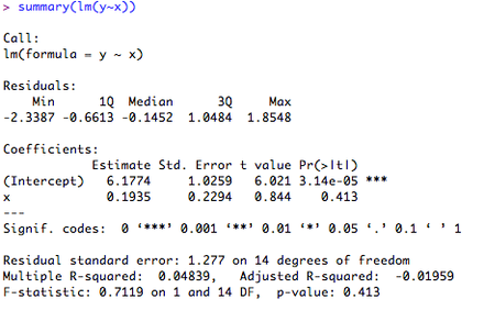
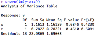
Consider the regression we carried out previously (y ~ x). Now, we add a second continuous variable (z) to the regression to make y ~ x + z. What we want to know is the unique amount of variance accounted for by variable 'x'. If we ask R for the summary of the lm model, this will give us the overall R², but as we need individual values, we need to ask R to give us a little more information. We can do this by asking for the ANOVA table of the regression:

This table tells us the Sum of Squares (Sum Sq. in the table above) for each of our predictors, so this will allow us to work out the individual R² values we need.

As with a simple regression, Cohen (1988) suggests f² values of 0.02, 0.15, and 0.35 represent small, medium, and large effect sizes, respectively.

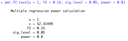
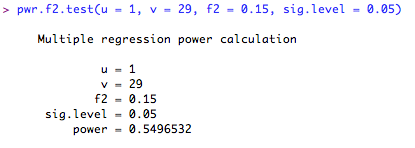
Calculate sample size:

Once we have the effect size, we can calculate the required sample size. In R, the basic command is:

where u is the numerator degrees of freedom (usually the number of levels of a factor minus 1, or simply '1' for a continuous variable) and v is the denominator degrees of freedom (is the sample size minus the numerator degrees of freedom).  Let's say for the above experiment we have one continuous predictor, and we are expecting a medium effect size, but we are not sure how many subjects we will need. To calculate the required sample size in R we would type:

As you will see, I left out the 'v = ...' command, as this is the value that I want R to calculate for me. It would seem that with this effect size, if I want to be 80% confident that I will get a significant result, I will need ~53 subjects (v ~ 52, so I need v + u subjects, which is ~53). What happens if I only have 30 subjects? Let's ask R:

According to this analysis, if I only have 30 subjects, I can only be 55% confident that I will detect a significant result given this effect size. Time to redesign the experiment I think!

In a regression model where the factor is continuous (e.g., units of alcohol consumed) the numerator degrees of freedom will be 1. However, there may be further factors, including, for example, categorical factors. Consider an experiment with a typical analysis of covariance (ANCOVA) design, where there is one categorical factor that has n levels, and one continuous covariate. Here we would need to calculate the unique effect size for the factor of interest (presumably the categorical factor) as described above for models with more than one factor (see previous section on 'Calculating Effect Size').

This is a little complicated, so let's try an example in R. First, we type our model into R, and ask for the ANOVA table so we can see the sums of squares estimates.

So if we want to use this for power analysis, we are going to want to know the variance of our response accounted for by our factor, while controlling for the effects of our covariate. This is important to think about, as a covariate (assuming it is a randomly distributed variable, as it should be!!) will not be the same every time we run this experiment!

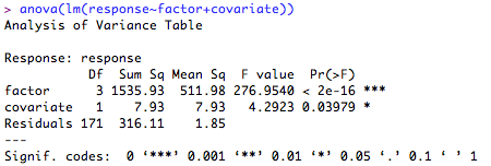
Imagine, for example, our factor is 'region where the subject lives' (i.e., North, South, East, West), our covariate is 'Body Mass Index', and our response is 'Units of Alcohol consumed in a week'. So we want to know how many units are consumed as a function of location, but we want to control for the effects of BMI. As you can probably see, we can select on the basis of where someone lives to repeat this, but we are unlikely to get the same BMIs corresponding to the same unites of alcohol again, so we need to partition this out of the effect size calculation.

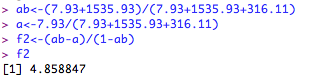
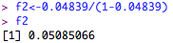
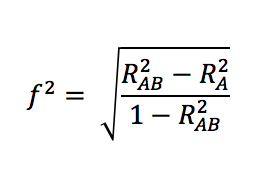
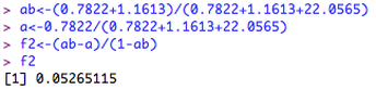
Using the nomenclature above, let's call the variance of our categorical factor 'B' and the total variance of our factor and covariate 'AB'. Let's type this into R:

Now we put the results into the pwr calculation:

You probably don't need to worry too much about the effect of the covariate in this model!

Return to previous page