As we talked about previously, usually the 'sig.level' = 0.05 and 'power' = 0.8. In an ideal world, the power will be 0.8, which means that you have an 80% chance of detecting a significant result if one exists.
Calculate effect size:
For chi-squared tests, the effect size, w, is calculated by the following
equation:
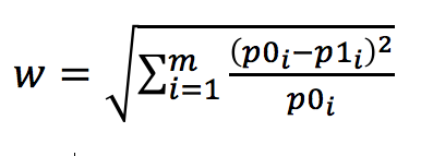
where p0i is the
probability
in the ith cell under the null hypothesis and p1i is the probability
in the ith cell under the alternative hypothesis. In
R, there are functions in the pwr library to calculate this effect size
(ES.w1), and the w statistic
for 2-way contingency tables (ES.w2).
If you have four probabilities under the alternative hypothesis (0.3, 0.4, 0.2, 0.1) and four under the null hypothesis (0.25, 0.25, 0.25, 0.25), type into R:
If you have four probabilities under the alternative hypothesis (0.3, 0.4, 0.2, 0.1) and four under the null hypothesis (0.25, 0.25, 0.25, 0.25), type into R:
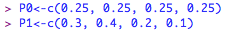
and then calculate the effect size w1:
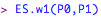
If you have a two-way contingency table e.g.,
this can be entered into R as a matrix:
| A |
B |
C |
D |
|
| a |
0.225 |
0.125 |
0.125 |
0.125 |
| b |
0.160 |
0.160 |
0.040 |
0.040 |
this can be entered into R as a matrix:
Then, the effect size can be calculated as:
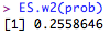
Cohen suggests that w values of 0.1, 0.3, and 0.5 represent small, medium, and large effect sizes respectively.
Calculate sample size:
Calculating the required sample size is the same, regardless of which effect size you have. The basic command in R for calculating the required sample size for a chi-squared test is:

where 'w' is the effect size calculated above, 'N' is the total sample size (number of observations), 'df' is the degrees of freedom (i.e., the number of cells minus one, and the number of columns minus 1), 'sig.level' is the required significance level (i.e., p < 0.05) and 'power' is the observed or required power of the design, given the effect size w.
For example, say you were planning to run an experiment looking at the proportion of a population of animals showing four distinct phenotypes. You are expecting a medium effect size, based on pilot data and you want to be 80% confident that you will detect this effect at the p = 0.05 cut-off. You would therefore type the following into R (note that I omit the 'N = ...' command, as this is what I want R to calculate for me):
For example, say you were planning to run an experiment looking at the proportion of a population of animals showing four distinct phenotypes. You are expecting a medium effect size, based on pilot data and you want to be 80% confident that you will detect this effect at the p = 0.05 cut-off. You would therefore type the following into R (note that I omit the 'N = ...' command, as this is what I want R to calculate for me):
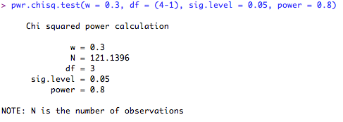
This means that in order to be 80% confident of detecting the effect, I will need 121 subjects. What if I only have 90 subjects? How confident can I be of detecting a significant result? Let's ask R. Note that this time, I leave the 'power = ...' command out, and enter the number of subjects I have in the 'N = ...' space.
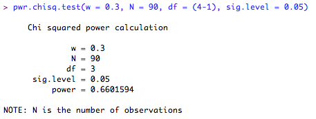
According to this, I can only be 66% confident that I will detect the effect given the sample size I have at my disposal. Time to re-design the experiment I think!
