T-tests and non-parametric equivalents
So, your experiment has: 1) two independent groups (e.g., wild-type vs mutant) and you are collecting continuous data at one time point (e.g., escape latency), OR 2) continuous data from one group of subjects, collected at two time points (e.g., reaction time before and after administration of a drug) OR 3) continuous data from one group of subjects, or at one time point, that is being compared against a population when we have limited information about the population (e.g., we may only know the population mean). By now you should have entered your data, and imported the data into R ready for analysis. Once you have done this, the first thing you need to do is to examine your data to check the best type of test to use.
T-tests are pretty robust, even if there is slight deviation from normality. In this sense, it is often not worth carrying out transformations on data prior to carrying out a t-test. If the data are clearly non-normal (i.e., the tails are extremely heavy) it is probably best to do a non-parametric wilcoxon test (see below) instead to be on the safe side. One situation where you need to be especially careful is where the sample size is very small. If this is the case (i.e., n ≥ 10) I would suggest you err on the side of caution, and carry out a non-parametric equivalent test.
In other tests (ANOVA, regression, etc.) we will examine the error distribution to ensure that the residuals are normally distributed. This is a condition for linear models. T-tests are slightly different in that they are testing the null hypothesis that the distributions of the two levels of the independent variable are the same, so as long as the variance is the same (t-tests require homoscedasticity). This is really important, so let's look at that first.
Tests of homoscedasticity (equality of variance)
This test will be necessary for independent-samples t-tests (paired t-test measures the differences between each pair, so this is irrelevant).
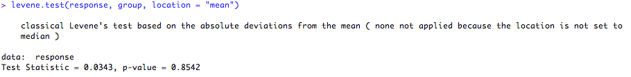
The most common test of equality of variances is called the Levene's test, which tests absolute deviations of observations from the corresponding group mean. There is a slightly more robust equivalent called the Brown-Forsythe test, which applies the Levene test to the median, instead of the mean. Which one of these you choose typically will depend on the distribution (i.e., if you are slightly concerned about the distribution, maybe go with the Brown-Forsythe test). This is really easy to carry out in R, but you will need to download a package called 'lawstat' the first time you use it. Luckily, this package does both of the above tests very straight-forwardly. Don't forget the test examples I have shown below relate to 'independent samples t-tests' (2 groups, one time-point).
The most common test of equality of variances is called the Levene's test, which tests absolute deviations of observations from the corresponding group mean. There is a slightly more robust equivalent called the Brown-Forsythe test, which applies the Levene test to the median, instead of the mean. Which one of these you choose typically will depend on the distribution (i.e., if you are slightly concerned about the distribution, maybe go with the Brown-Forsythe test). This is really easy to carry out in R, but you will need to download a package called 'lawstat' the first time you use it. Luckily, this package does both of the above tests very straight-forwardly. Don't forget the test examples I have shown below relate to 'independent samples t-tests' (2 groups, one time-point).

Next, make the package active:

Now, activate the datasheet you are working on, and you are ready to carry out the test.
In this example, let's suppose that you have a response variable 'response' and a group variable 'group'. First, we will try the levene test:
Now, let's try the Brown-Forsythe test on the same data:
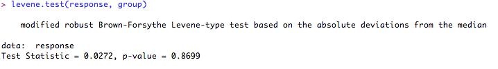
As these are testing the NULL HYPOTHESIS that the variances of the difference levels of 'group' are equal, if the 'p' value is < 0.05, we must assume that the variances are not equal. If the 'p' value is > 0.05 (as it is here) we have no evidence to reject the null hypothesis, so we can assume the variances are equal. In either case, we will use a version of the t-test that allows for this. Again, in R this is pretty simple as the R t-test defaults to this more conservative calculation anyway!
Check for normality
Before we plough on with the analysis, you need to check the distribution of the data. There are various ways to do this, and we will go through some a couple of them here. For other kinds of analysis (where regressions are being calculated) you will examine the distribution of the residuals, rather than the raw data. For t-tests, there are no residuals in this sense, as the t-test is testing the null hypothesis that the means (of two normally distributed populations) are the same.
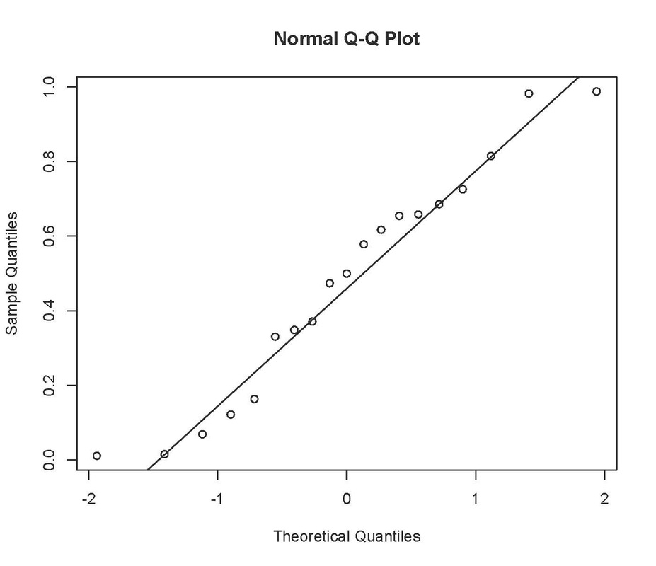
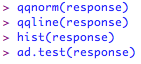
The first thing to do is to examine the distributions of the populations. The two most common ways of doing this are using normal quantile plots (often referred to as Q-Q plots) or histograms. Type both of these lines into R (nb., 'data' is the name of the datafile that you have already imported into R).
The first thing to do is to examine the distributions of the populations. The two most common ways of doing this are using normal quantile plots (often referred to as Q-Q plots) or histograms. Type both of these lines into R (nb., 'data' is the name of the datafile that you have already imported into R).

will produce:
You can then do the same for group b:

If the observations follow approximately a normal distribution, the Q-Q plot should be roughly a straight line without too much deviation. It is not a precise science! In the plot above, although there are a couple of 'outliers', most of the points are in a straight line so this should be OK without transformation. As I stated previously, small deviations from normality should not present a problem for t-tests, as long as the variance between the samples is equal.
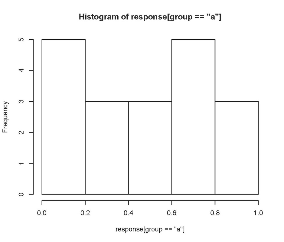
You can also plot histograms. For example:
You can also plot histograms. For example:

will produce:
and
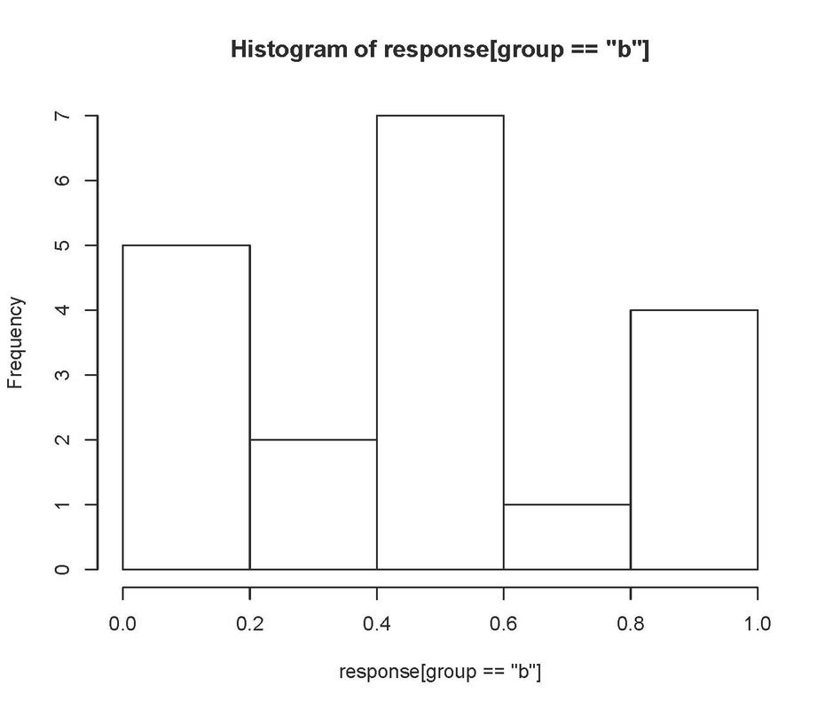
Neither of these look particularly normal! Having said that the Q-Q plot looks pretty good, so I would probably be happy with leaving these data untransformed.
There are various calculations that can be carried out to test normality, but there is much debate in the literature as to whether these tests are any good (see below). One such example available in R is the Anderson Darling test, which tests the null hypothesis that your variable is accounted for by a normal distribution. In order to do this test in R, you will need to install a package and invoke it:
There are various calculations that can be carried out to test normality, but there is much debate in the literature as to whether these tests are any good (see below). One such example available in R is the Anderson Darling test, which tests the null hypothesis that your variable is accounted for by a normal distribution. In order to do this test in R, you will need to install a package and invoke it:


Now you can run the test on your groups:
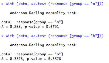
Well, that looks ok! According to this test there is no evidence to assume that either of the group distributions deviate from normality.
A word of warning, however. As the test is very accurate, for very large sample sizes the results may be misleading (see here for an example!).
In sum, I would always recommend looking at the Q-Q plots and the histograms. The A-D test and those like it can be useful in some instances, but use caution!!
If you are carrying out a paired or a 1-sample t-test, all you need to do is to check the distribution of the response variable. The reason for this in the case of a paired t-test is that the test is carried out on the differences between each pair, rather than each group as independent.
For paired t-tests, you should also check the correlation of the conditions, as if they are not correlated you should probably carry out an independent samples test (although it might suggest to me that there was a problem with my experiment). You can do this by typing (where 'condition' represents the time points, and 'response' is the dependent variable:

Run a t-test
Once you are happy that the data are normal and you know if the variances are equal, you are ready to run the test.
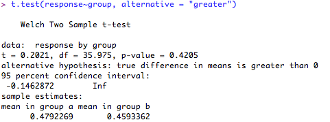
In all cases for the examples below, I will be carrying out "two-tailed tests". In other words, the 'p' value will be calculated based on both extremes of the distribution tails. This is more conservative than the alternative "one tailed tests" (learn more). If you wish to carry out a "one-tailed test" instead, you need to add the following term to your R code (the example below is for an independent samples t-test, but will work with any of the examples below).
First for a one-tailed hypothesis that the difference between the groups will be greater than '0':
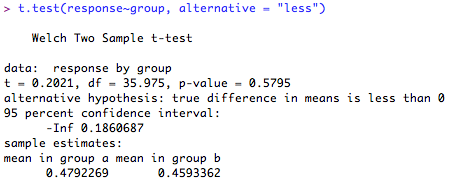
Or less than '0':
1. Independent samples t-test for samples with equal variances (normal distribution assumed)
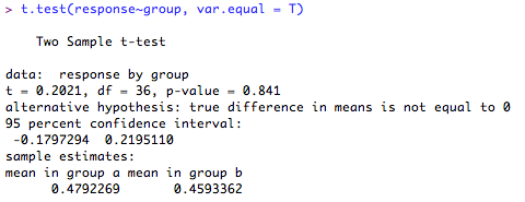
The test output give the test statistic, the degrees of freedom, 95% confidence intervals, group score estimates and the 'p' value. It also (helpfully!) tells you what the alternative hypothesis is (hint: this will usually be that the difference in means is ≠ 0!). Here, the difference in the means is not significantly different from '0' (p = 0.84) so you cannot reject the null hypothesis.
2. Independent samples t-test for samples with unequal variances (normal distribution assumed).
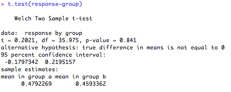
The test output give the test statistic, the degrees of freedom, 95% confidence intervals, group score estimates and the 'p' value. It also (helpfully!) tells you what the alternative hypothesis is (hint: this will usually be that the difference in means is ≠ 0!). Notice that the output is similar to the test with equal variances, but the degrees of freedom are slightly adjusted to account for the unequal variance (it works out the variances separately, not together). Here, the difference in the means is not significantly different from '0' (p = 0.84) so you cannot reject the null hypothesis.
3. Paired t-test for samples (normal distribution assumed).
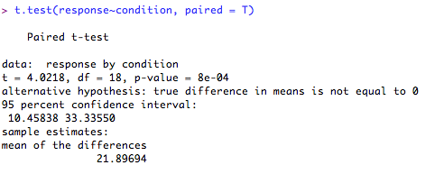
The test output give the test statistic, the degrees of freedom, 95% confidence intervals, condition score estimates and the 'p' value. It also (helpfully!) tells you what the alternative hypothesis is (hint: this will usually be that the difference in means is ≠ 0!).Finally, it tells you the mean of the differences between the conditions (rather than the mean of 'condition a' and 'condition b'). Here, the difference between your conditions is significantly different from '0' (p = 8e-04 [this means p = 0.00008]), so you can reject your null hypothesis in favour of the alternative hypothesis.
4. Independent-samples test (serious deviation from normality)
If you find a serious deviation from normality, you can choose to use a Wilcoxon rank-sum test (sometimes called Mann-Whitney U test).
If you find a serious deviation from normality, you can choose to use a Wilcoxon rank-sum test (sometimes called Mann-Whitney U test).
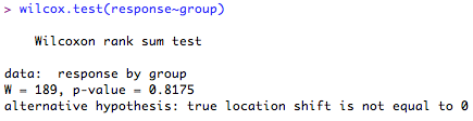
The output gives you the test statistic (called 'W') and the 'p' value. Here, the differences between the locations of the ranks of the scores in each group is not significantly different from '0' (p = 0.8175) so you cannot reject your null hypothesis.
5. Paired-samples test (serious deviation from normality)
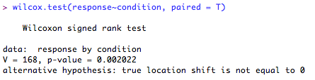
The output gives you the test statistics (called 'V') and the 'p' value. Here, the difference between the ranked differences of the scores in each of the conditions is significantly different from '0' (p = 0.002) so you can reject the null hypothesis in favour of the alternative hypothesis.
6. One sample t-test, testing the sample mean against an assumed population mean of 0.5 (normal distribution assumed).
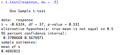
Here, the output tells you the test statistic (t), the degrees of freedom (df) and the 'p' value. Note that here, R tells you that your alternative hypothesis is that the difference in mean ≠ 0.5. Finally it tells you the sample mean. In this case, the sample mean (0.469) is not significantly different from the assumed population mean (0.5) (p = 0.531) so you cannot reject the null hypothesis.
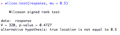
7. One-sample test, testing the sample median against an assumed population median of 0.5 (serious deviation from normality)